cuNumeric.jl 
Collaborators
- Carnegie Mellon University
Ethan Meitz - Los Alamos National Laboratory
Pat McCormick - NVIDIA
Wonchan Lee
Note: this page is outdated. The benchmarks and implementation details below reflect an early version of cuNumeric.jl. A paper, cuNumeric.jl: Automated Performant Multi-GPU Numerical Computing for Julia, has been submitted to IPDPS. For current performance results, see the up-to-date benchmark results.
cuNumeric.jl enables heterogeneous distributed code execution with minimal effort. The core type is the NDArray- a drop-in replacement for the Base.Array within Julia. Some of the key differences include:
- operations are broadcast by default
- slices are always view references
- important to avoid scalar indexing to achieve decent performance
Legate
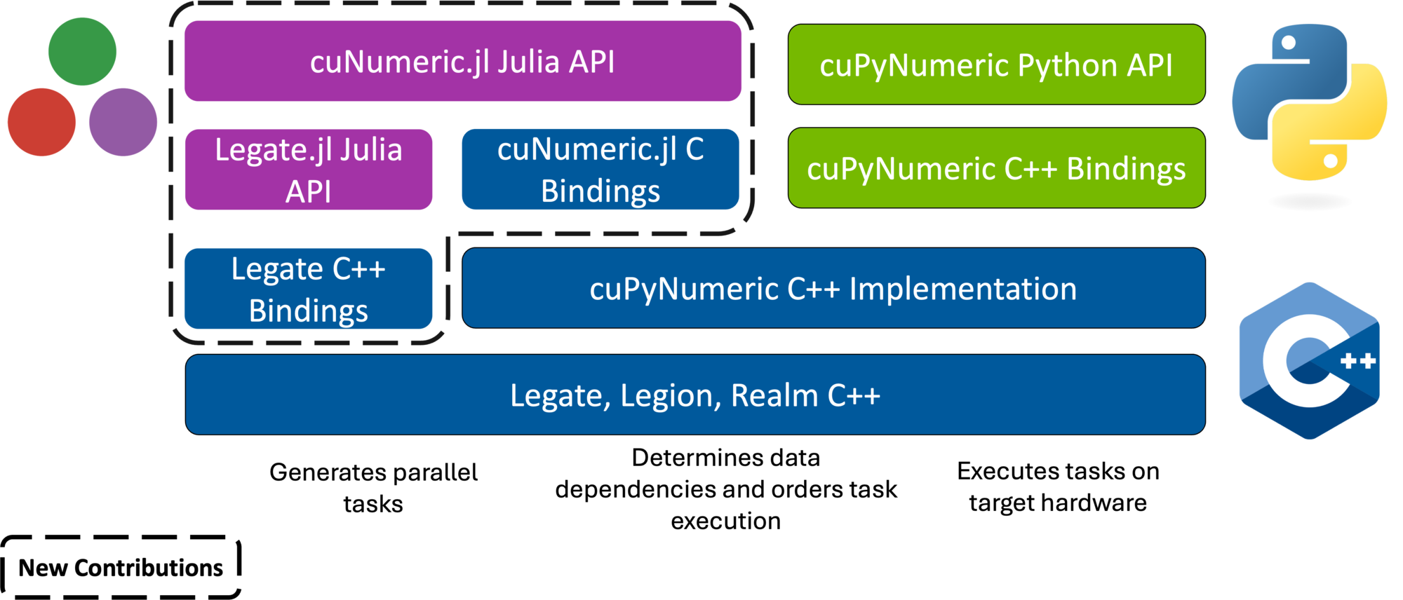
This library is enabled through the Legate runtime. Legate provides data and task management abstractions to enable the efficient implementation of complex library APIs. The work has mainly been focused on the top Python libraries with cuPyNumeric, Legate Sparse, Legate Dataframe, etc. However, our work is to bring this novel infrastructure to the Julia Language ecosystem.
How does Legate work?
All libraries share common data representation and task management. Different Legate programs can issue API calls to add to a task graph.
Legate stores implement common array protocols, allowing task bodies to reuse existing single processor libraries (e.g., NumPy, CuPy, or Numba)
Our contributions
Benchmarks
These results are outdated. See the current benchmark results.
N = 1000
A = cuNumeric.rand(Float32, N, N)
B = cuNumeric.rand(Float32, N, N)
C = cuNumeric.zeros(Float32, N, N)
mul!(C, A, B)
GEMM
First, we start off with a GEMM that scales to 8xA100 GPUs.
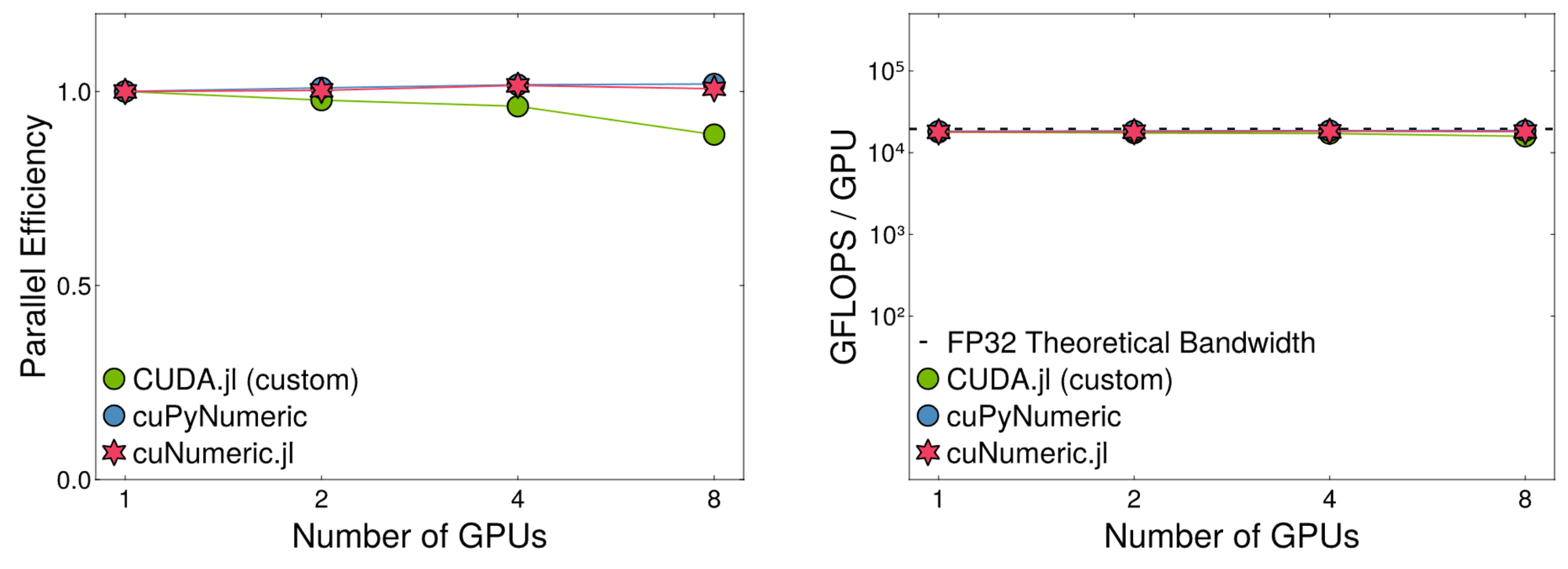 We see that GEMM weak scales and matches cuPyNumeric. Additionally, we notice our naive CUDA.jl implementation is falling behind in terms of parallel efficiency.
Monte Carlo
integrand = (x) -> exp(-square(x))
N = 1_000_000
x_max = 5.0
domain = [-x_max, x_max]
Ω = domain[2] - domain[1]
samples = Ω*cuNumeric.rand(NDArray, N) - x_max
estimate = (Ω/N) * sum(integrand(samples))
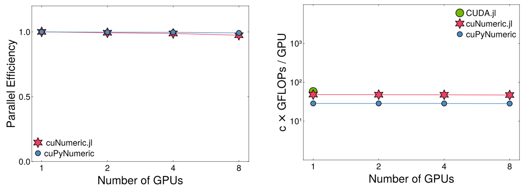 Using the same 8xA100 GPUs, we see Monte Carlo integration matches cuPyNumeric in parallel efficiency. Also, we are able to achieve speedup relative to cuPyNumeric in terms of FLOPS. This is due to the several layers of Python that cuPyNumeric handles while we rely directly on a minimum Julia front end that calls directly into C++.
Gray Scott Reaction-Diffusion
N = 100
u = cuNumeric.ones((N, N))
v = cuNumeric.ones((N, N))
for i in iters
   F_u = ((u[2:(end - 1), 2:(end - 1)] .* (v[2:(end - 1), 2:(end - 1)]
       .* v[2:(end - 1), 2:(end - 1)])) - (f+k)*v[2:(end - 1), 2:(end - 1)])
   #.... more physics
   #.... update u and v
end
At first this failed to run. During the construction of our task graph, Legate failed to map the cuNumeric.jl program. We rely on notifications from finalizer calls to notify the runtime the lifetimes of objects. However, we were disrupted with the heap heuristics of the mark and sweep garbage collector within Julia.
using CUDA, Profile
arr = CUDA.ones(Float32, 10_000_000)
Profile.take_heap_snapshot()
Base.summarysize(arr) # 184
Running the code above, the 10 million element array of Float32s is about 40 Mb. However, Julia sees only 184 bytes in the heap snapshot.
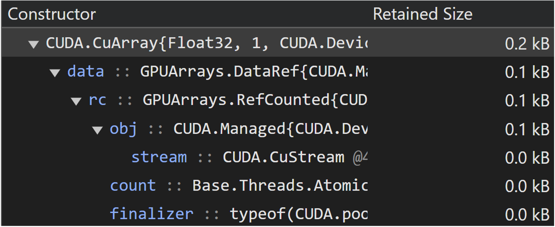
Due to this lack of heap usage, the Julia garbage collector never gets called during the execution of a cuNumeric.jl program. This is the reason why the above Gray-Scott reaction-diffusion code fails to run.
We looked into other existing backends that deal with external memory references. In short, they have three phases of the GC:
- Calculate array memory footprint in the constructor
- Manually call GC based on a memory pressure heuristic
- Try-catch on allocation to avoid out-of-memory errors
Two things that make this above approach difficult for cuNumeric.jl:
- Deferred execution model conceals Julia object's physical size at creation
- Runtime cannot recover from failed mapping allocation
In order to run Gray-Scott, we experimented with manually inserting GC.gc() calls within the main loop body. We varied the iteration interval with values 1,3,6.
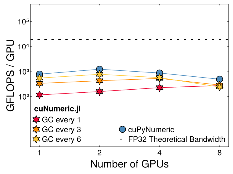
As we decrease the number of garbage collection invocations, we approach cuPyNumeric's performance on the Gray-Scott example. However, there is still a noticeable gap in performance between GC every 6 and cuPyNumeric. The application fails to run at an interaction interval of 7.
We decided to create a custom GC heap heuristic similar to the methodology described above.
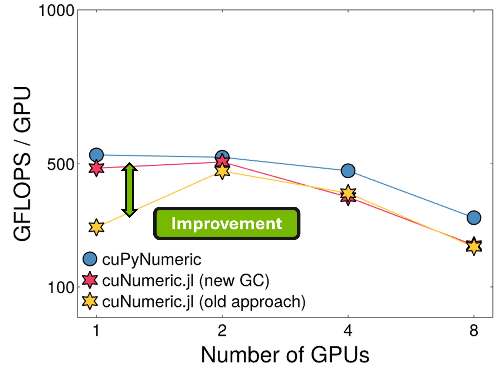
Performance improves substantially for GPU counts of 1 and 2; however, there is a large gap for GPU counts of 4 and 8. This is future work.
Performance
One thing you may notice is that cuPyNumeric and cuNumeric.jl performance results are far from the theoretical FP32 bandwidth.
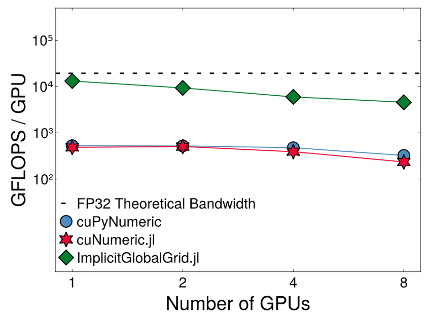
ImplicitGlobalGrid.jl [1] performs substantially better than us. This library is a specialized stencil-based PDE solver. They support multi-node heterogeneous execution with minimal code changes.
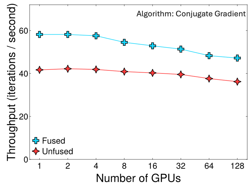
This work above is done by the Legate team. The work reveals that kernel task fusion can provide an average of a 2x speedup (up to 10x) on cuPyNumeric task workloads. As we are using the same infrastructure, we believe this is a huge performance bottleneck for operator-by-operator intensive workloads. As we don't have kernel task fusion, we aim to support custom CUDA.jl kernel registration. These kernels can act as "fused" variants to compare against potential speedups we can get from operator fusion.
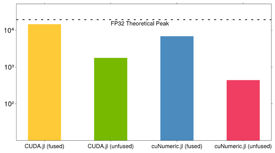
CUDA.jl and cuNumeric.jl support both custom kernels and operator-by-operator support. This benchmark is a 1D variant of the Gray Scott heat diffusion. In both models, the custom CUDA fused kernels perform much better then the unfused operator-by-operator counterparts. In this example, CUDA.jl (fused) performs better than cuNumeric.jl (fused). This is due to overheads in our backend. These overheads get amortized as GPU count increases. We enable distributed execution compared to CUDA.jl. This might lead us to get better performance for the full Gray-Scott simulation approaching the FP32 theoretical peak.
Currently, we have ongoing backend enhancements for multi-dimensional workloads and multi-GPU execution
Custom kernel registration
function kernel_add(a, b, c, N)
   i = (blockIdx().x - 1i32) * blockDim().x + threadIdx().x
   if i <= N
       @inbounds c[i] = a[i] + b[i]
   end
   return nothing
end

N = 1024
threads = 256
blocks = cld(N, threads)

a = cuNumeric.full(N, 1.0f0)
b = cuNumeric.full(N, 2.0f0)
c = cuNumeric.ones(Float32, N)

task = cuNumeric.@cuda_task kernel_add(a, b, c, UInt32(1))

cuNumeric.@launch task=task threads=threads blocks=blocks inputs=(a, b) outputs=c scalars=UInt32(N)